Elementary flow

In the larger context of the Navier-Stokes equations (and especially in the context of potential theory), elementary flows are basic flows that can be combined, using various techniques, to construct more complex flows. In this article the term "flow" is used interchangeably with the term "solution" due to historical reasons.

The techniques involved to create more complex solutions can be for example by superposition, by techniques such as topology or considering them as local solutions on a certain neighborhood, subdomain or boundary layer and to be patched together. Elementary flows can be considered the basic building blocks (fundamental solutions, local solutions and solitons) of the different types of equations derived from the Navier-Stokes equations. Some of the flows reflect specific constraints such as incompressible or irrotational flows, or both, as in the case of potential flow, and some of the flows may be limited to the case of two dimensions.^[1]

Due to the relationship between fluid dynamics and field theory, elementary flows are relevant not only to aerodynamics but to all field theory in general. To put it in perspective boundary layers can be interpreted as topological defects on generic manifolds, and considering fluid dynamics analogies and limit cases in electromagnetism, quantum mechanics and general relativity one can see how all these solutions are at the core of recent developments in theoretical physics such as the ads/cft duality, the SYK model, the physics of nematic liquids, strongly correlated systems and even to quark gluon plasmas.

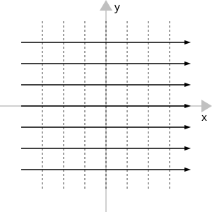
For steady-state, spatially uniform flow of a fluid in the xy plane, the velocity vector is

${\displaystyle \mathbf {v} =v_{0}\cos(\theta _{0})\,\mathbf {e} _{x}+v_{0}\sin(\theta _{0})\,\mathbf {e} _{y}}$

where

${\displaystyle v_{0}}$ is the absolute magnitude of the velocity (i.e., ${\displaystyle v_{0}=|\mathbf {v} |}$);

${\displaystyle \theta _{0}}$ is the angle the velocity vector makes with the positive x axis (${\displaystyle \theta _{0}}$ is positive for angles measured in a counterclockwise sense from the positive x axis); and

${\displaystyle \mathbf {e} _{x}}$ and ${\displaystyle \mathbf {e} _{y}}$ are the unit basis vectors of the xy coordinate system.

Because this flow is incompressible (i.e., ${\displaystyle \nabla \cdot \mathbf {v} =0}$) and two-dimensional, its velocity can be expressed in terms of a stream function, ${\displaystyle \psi }$:

${\displaystyle v_{x}={\frac {\partial \psi }{\partial y}}}$

${\displaystyle v_{y}=-{\frac {\partial \psi }{\partial x}}}$

where

${\displaystyle \psi =\psi _{0}-v_{0}\sin(\theta _{0})\,x+v_{0}\cos(\theta _{0})\,y}$

and ${\displaystyle \psi _{0}}$ is a constant.

In cylindrical coordinates:

${\displaystyle v_{r}=-{\frac {1}{r}}{\frac {\partial \psi }{\partial \theta }}}$

${\displaystyle v_{\theta }={\frac {\partial \psi }{\partial r}}}$

and

${\displaystyle \psi =\psi _{0}+v_{0}\,r\sin(\theta -\theta _{0})}$

This flow is irrotational (i.e., ${\displaystyle \nabla \times \mathbf {v} =\mathbf {0} }$) so its velocity can be expressed in terms of a potential function, ${\displaystyle \phi }$:

${\displaystyle v_{x}=-{\frac {\partial \phi }{\partial x}}}$

${\displaystyle v_{y}=-{\frac {\partial \phi }{\partial y}}}$

where

${\displaystyle \phi =\phi _{0}-v_{0}\cos(\theta _{0})\,x-v_{0}\sin(\theta _{0})\,y}$

and ${\displaystyle \phi _{0}}$ is a constant.

In cylindrical coordinates

${\displaystyle v_{r}={\frac {\partial \phi }{\partial r}}}$

${\displaystyle v_{\theta }={\frac {1}{r}}{\frac {\partial \phi }{\partial \theta }}}$

${\displaystyle \phi =\phi _{0}-v_{0}\,r\cos(\theta -\theta _{0})}$

The case of a vertical line emitting at a fixed rate a constant quantity of fluid Q per unit length is a line source. The problem has a cylindrical symmetry and can be treated in two dimensions on the orthogonal plane.

Line sources and line sinks (below) are important elementary flows because they play the role of monopole for incompressible fluids (which can also be considered examples of solenoidal fields i.e. divergence free fields). Generic flow patterns can be also de-composed in terms of multipole expansions, in the same manner as for electric and magnetic fields where the monopole is essentially the first non-trivial (e.g. constant) term of the expansion.

This flow pattern is also both irrotational and incompressible.

This is characterized by a cylindrical symmetry:

${\displaystyle \mathbf {v} =v_{r}(r)\mathbf {e} _{r}}$

Where the total outgoing flux is constant

${\displaystyle \int _{S}\mathbf {v} \cdot d\mathbf {S} =\int _{0}^{2\pi }(v_{r}(r)\,\mathbf {e} _{r})\cdot (\mathbf {e} _{r}\,r\,d\theta )=\!2\pi \,r\,v_{r}(r)=Q}$

Therefore,

${\displaystyle v_{r}={\frac {Q}{2\pi r}}}$

This is derived from a stream function

${\displaystyle \psi (r,\theta )=-{\frac {Q}{2\pi }}\theta }$

or from a potential function

${\displaystyle \phi (r,\theta )=-{\frac {Q}{2\pi }}\ln r}$

The case of a vertical line absorbing at a fixed rate a constant quantity of fluid Q per unit length is a line sink. Everything is the same as the case of a line source a part from the negative sign.

${\displaystyle v_{r}=-{\frac {Q}{2\pi r}}}$

This is derived from a stream function

${\displaystyle \psi (r,\theta )={\frac {Q}{2\pi }}\theta }$

or from a potential function

${\displaystyle \phi (r,\theta )={\frac {Q}{2\pi }}\ln r}$

Given that the two results are the same a part from a minus sign we can treat transparently both line sources and line sinks with the same stream and potential functions permitting Q to assume both positive and negative values and absorbing the minus sign into the definition of Q.

If we consider a line source and a line sink at a distance d we can reuse the results above and the stream function will be

${\displaystyle \psi (\mathbf {r} )=\psi _{Q}(\mathbf {r} -\mathbf {d} /2)-\psi _{Q}(\mathbf {r} +\mathbf {d} /2)\ \simeq \mathbf {d} \cdot \nabla \psi _{Q}(\mathbf {r} )}$

The last approximation is to the first order in d.

Given

${\displaystyle \mathbf {d} =d[\cos(\theta _{0})\mathbf {e} _{x}+\sin(\theta _{0})\mathbf {e} _{y}]=d[\cos(\theta -\theta _{0})\mathbf {e} _{r}+\sin(\theta -\theta _{0})\mathbf {e} _{\theta }]}$

It remains

${\displaystyle \psi (r,\theta )=-{\frac {Qd}{2\pi }}{\frac {\sin(\theta -\theta _{0})}{r}}}$

The velocity is then

${\displaystyle v_{r}(r,\theta )={\frac {Qd}{2\pi }}{\frac {\cos(\theta -\theta _{0})}{r^{2}}}}$

${\displaystyle v_{\theta }(r,\theta )={\frac {Qd}{2\pi }}{\frac {\sin(\theta -\theta _{0})}{r^{2}}}}$

And the potential instead

${\displaystyle \phi (r,\theta )={\frac {Qd}{2\pi }}{\frac {\cos(\theta -\theta _{0})}{r}}}$

This is the case of a vortex filament rotating at constant speed, there is a cylindrical symmetry and the problem can be solved in the orthogonal plane.

Dual to the case above of line sources, vortex lines play the role of monopoles for irrotational flows.

Also in this case the flow is also both irrotational and incompressible and therefore a case of potential flow.

This is characterized by a cylindrical symmetry:

${\displaystyle \mathbf {v} =v_{\theta }(r)\,\mathbf {e} _{\theta }}$

Where the total circulation is constant for every closed line around the central vortex

${\displaystyle \oint \mathbf {v} \cdot d\mathbf {s} =\int _{0}^{2\pi }(v_{\theta }(r)\,\mathbf {e} _{\theta })\cdot (\mathbf {e} _{\theta }\,r\,d\theta )=\!2\pi \,r\,v_{\theta }(r)=\Gamma }$

and is zero for any line not including the vortex.

Therefore,

${\displaystyle v_{\theta }={\frac {\Gamma }{2\pi r}}}$

This is derived from a stream function

${\displaystyle \psi (r,\theta )={\frac {\Gamma }{2\pi }}\ln r}$

or from a potential function

${\displaystyle \phi (r,\theta )=-{\frac {\Gamma }{2\pi }}\theta }$

Which is dual to the previous case of a line source

Given an incompressible two-dimensional flow which is also irrotational we have:

${\displaystyle \nabla ^{2}\psi =0}$

Which is in cylindrical coordinates ^[2]

${\displaystyle {\frac {1}{r}}{\frac {\partial }{\partial r}}\left(r{\frac {\partial \psi }{\partial r}}\right)+{\frac {1}{r^{2}}}{\frac {\partial ^{2}\psi }{\partial \theta ^{2}}}=0}$

We look for a solution with separated variables:

${\displaystyle \psi (r,\theta )=R(r)\Theta (\theta )}$

which gives

${\displaystyle {\frac {r}{R(r)}}{\frac {d}{dr}}\left(r{\frac {dR(r)}{dr}}\right)=-{\frac {1}{\Theta (\theta )}}{\frac {d^{2}\Theta (\theta )}{d\theta ^{2}}}}$

Given the left part depends only on r and the right parts depends only on ${\displaystyle \theta }$, the two parts must be equal to a constant independent from r and ${\displaystyle \theta }$. The constant shall be positive^{[clarification needed]}. Therefore,

${\displaystyle r{\frac {d}{dr}}\left(r{\frac {d}{dr}}R(r)\right)=m^{2}R(r)}$

${\displaystyle {\frac {d^{2}\Theta (\theta )}{d\theta ^{2}}}=-m^{2}\Theta (\theta )}$

The solution to the second equation is a linear combination of ${\displaystyle e^{im\theta }}$ and ${\displaystyle e^{-im\theta }}$ In order to have a single-valued velocity (and also a single-valued stream function) m shall be a positive integer.

therefore the most generic solution is given by

${\displaystyle \psi =\alpha _{0}+\beta _{0}\ln r+\sum _{m>0}{\left(\alpha _{m}r^{m}+\beta _{m}r^{-m}\right)\sin {[m(\theta -\theta _{m})]}}}$

The potential is instead given by

${\displaystyle \phi =\alpha _{0}-\beta _{0}\theta +\sum _{m\mathop {>} 0}{(\alpha _{m}r^{m}-\beta _{m}r^{-m})\cos {[m(\theta -\theta _{m})]}}}$

• Fitzpatrick, Richard (2017), Theoretical fluid dynamics, IOP science, ISBN 978-0-7503-1554-8
• Faber, T.E. (1995), Fluid Dynamics for Physicists, Cambridge university press, ISBN 9780511806735

Specific

• Batchelor, G.K. (1973), An introduction to fluid dynamics, Cambridge University Press, ISBN 978-0-521-09817-5
• Chanson, H. (2009), Applied Hydrodynamics: An Introduction to Ideal and Real Fluid Flows, CRC Press, Taylor & Francis Group, Leiden, The Netherlands, 478 pages, ISBN 978-0-415-49271-3
• Lamb, H. (1994) [1932], Hydrodynamics (6th ed.), Cambridge University Press, ISBN 978-0-521-45868-9
• Milne-Thomson, L.M. (1996) [1968], Theoretical hydrodynamics (5th ed.), Dover, ISBN 978-0-486-68970-8

• Richard Fitzpatrick University of Texas, Austin (2017). "Fluid Mechanics". University of Texas, Austin. Retrieved 2018-02-07.

• (c) Aerospace, Mechanical & Mechatronic Engg. 2005 University of Sydney (2005). "Elements of Potential Flow". University of Sydney. Retrieved 2019-04-19.{{cite web}}: CS1 maint: numeric names: authors list (link)