Periodic points of complex quadratic mappings

This article describes periodic points of some complex quadratic maps. A map is a formula for computing a value of a variable based on its own previous value or values; a quadratic map is one that involves the previous value raised to the powers one and two; and a complex map is one in which the variable and the parameters are complex numbers. A periodic point of a map is a value of the variable that occurs repeatedly after intervals of a fixed length.

These periodic points play a role in the theories of Fatou and Julia sets.

Let

${\displaystyle f_{c}(z)=z^{2}+c\,}$

be the complex quadric mapping, where ${\displaystyle z}$ and ${\displaystyle c}$ are complex numbers.

Notationally, ${\displaystyle f_{c}^{(k)}(z)}$ is the ${\displaystyle k}$-fold composition of ${\displaystyle f_{c}}$ with itself (not to be confused with the ${\displaystyle k}$th derivative of ${\displaystyle f_{c}}$)—that is, the value after the k-th iteration of the function ${\displaystyle f_{c}.}$ Thus

${\displaystyle f_{c}^{(k)}(z)=f_{c}(f_{c}^{(k-1)}(z)).}$

Periodic points of a complex quadratic mapping of period ${\displaystyle p}$ are points ${\displaystyle z}$ of the dynamical plane such that

${\displaystyle f_{c}^{(p)}(z)=z,}$

where ${\displaystyle p}$ is the smallest positive integer for which the equation holds at that z.

We can introduce a new function:

${\displaystyle F_{p}(z,f)=f_{c}^{(p)}(z)-z,}$

so periodic points are zeros of function ${\displaystyle F_{p}(z,f)}$: points z satisfying

${\displaystyle F_{p}(z,f)=0,}$

which is a polynomial of degree ${\displaystyle 2^{p}.}$

The degree of the polynomial ${\displaystyle F_{p}(z,f)}$ describing periodic points is ${\displaystyle d=2^{p}}$ so it has exactly ${\displaystyle d=2^{p}}$ complex roots (= periodic points), counted with multiplicity.

The multiplier (or eigenvalue, derivative) ${\displaystyle m(f^{p},z_{0})=\lambda }$ of a rational map ${\displaystyle f}$ iterated ${\displaystyle p}$ times at cyclic point ${\displaystyle z_{0}}$ is defined as:

${\displaystyle m(f^{p},z_{0})=\lambda ={\begin{cases}f^{p\prime }(z_{0}),&{\mbox{if }}z_{0}\neq \infty \\{\frac {1}{f^{p\prime }(z_{0})}},&{\mbox{if }}z_{0}=\infty \end{cases}}}$

where ${\displaystyle f^{p\prime }(z_{0})}$ is the first derivative of ${\displaystyle f^{p}}$ with respect to ${\displaystyle z}$ at ${\displaystyle z_{0}}$.

Because the multiplier is the same at all periodic points on a given orbit, it is called a multiplier of the periodic orbit.

The multiplier is:

• a complex number;
• invariant under conjugation of any rational map at its fixed point;^[1]
• used to check stability of periodic (also fixed) points with stability index ${\displaystyle abs(\lambda ).\,}$

A periodic point is^[2]

• attracting when ${\displaystyle abs(\lambda )<1;}$
  • super-attracting when ${\displaystyle abs(\lambda )=0;}$
  • attracting but not super-attracting when ${\displaystyle 0<abs(\lambda )<1;}$
• indifferent when ${\displaystyle abs(\lambda )=1;}$
  • rationally indifferent or parabolic if ${\displaystyle \lambda }$ is a root of unity;
  • irrationally indifferent if ${\displaystyle abs(\lambda )=1}$ but multiplier is not a root of unity;
• repelling when ${\displaystyle abs(\lambda )>1.}$

Periodic points

• that are attracting are always in the Fatou set;
• that are repelling are in the Julia set;
• that are indifferent fixed points may be in one or the other.^[3] A parabolic periodic point is in the Julia set.

Let us begin by finding all finite points left unchanged by one application of ${\displaystyle f}$. These are the points that satisfy ${\displaystyle f_{c}(z)=z}$. That is, we wish to solve

${\displaystyle z^{2}+c=z,\,}$

which can be rewritten as

${\displaystyle \ z^{2}-z+c=0.}$

Since this is an ordinary quadratic equation in one unknown, we can apply the standard quadratic solution formula:

${\displaystyle \alpha _{1}={\frac {1-{\sqrt {1-4c}}}{2}}}$ and ${\displaystyle \alpha _{2}={\frac {1+{\sqrt {1-4c}}}{2}}.}$

So for ${\displaystyle c\in \mathbb {C} \setminus \{1/4\}}$ we have two finite fixed points ${\displaystyle \alpha _{1}}$ and ${\displaystyle \alpha _{2}}$.

Since

${\displaystyle \alpha _{1}={\frac {1}{2}}-m}$ and ${\displaystyle \alpha _{2}={\frac {1}{2}}+m}$ where ${\displaystyle m={\frac {\sqrt {1-4c}}{2}},}$

we have ${\displaystyle \alpha _{1}+\alpha _{2}=1}$.

Thus fixed points are symmetrical about ${\displaystyle z=1/2}$.

Here different notation is commonly used:^[4]

${\displaystyle \alpha _{c}={\frac {1-{\sqrt {1-4c}}}{2}}}$ with multiplier ${\displaystyle \lambda _{\alpha _{c}}=1-{\sqrt {1-4c}}}$

and

${\displaystyle \beta _{c}={\frac {1+{\sqrt {1-4c}}}{2}}}$ with multiplier ${\displaystyle \lambda _{\beta _{c}}=1+{\sqrt {1-4c}}.}$

Again we have

${\displaystyle \alpha _{c}+\beta _{c}=1.}$

Since the derivative with respect to z is

${\displaystyle P_{c}'(z)={\frac {d}{dz}}P_{c}(z)=2z,}$

we have

${\displaystyle P_{c}'(\alpha _{c})+P_{c}'(\beta _{c})=2\alpha _{c}+2\beta _{c}=2(\alpha _{c}+\beta _{c})=2.}$

This implies that ${\displaystyle P_{c}}$ can have at most one attractive fixed point.

These points are distinguished by the facts that:

• ${\displaystyle \beta _{c}}$ is:
  • the landing point of the external ray for angle=0 for ${\displaystyle c\in M\setminus \left\{1/4\right\}}$
  • the most repelling fixed point of the Julia set
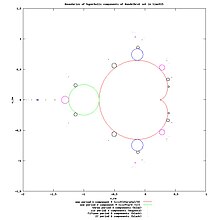
  • the one on the right (whenever fixed point are not symmetrical around the real axis), it is the extreme right point for connected Julia sets (except for cauliflower).^[5]
• ${\displaystyle \alpha _{c}}$ is:
  • the landing point of several rays
  • attracting when ${\displaystyle c}$ is in the main cardioid of the Mandelbrot set, in which case it is in the interior of a filled-in Julia set, and therefore belongs to the Fatou set (strictly to the basin of attraction of finite fixed point)
  • parabolic at the root point of the limb of the Mandelbrot set
  • repelling for other values of ${\displaystyle c}$

An important case of the quadratic mapping is ${\displaystyle c=0}$. In this case, we get ${\displaystyle \alpha _{1}=0}$ and ${\displaystyle \alpha _{2}=1}$. In this case, 0 is a superattractive fixed point, and 1 belongs to the Julia set.

We have ${\displaystyle \alpha _{1}=\alpha _{2}}$ exactly when ${\displaystyle 1-4c=0.}$ This equation has one solution, ${\displaystyle c=1/4,}$ in which case ${\displaystyle \alpha _{1}=\alpha _{2}=1/2}$. In fact ${\displaystyle c=1/4}$ is the largest positive, purely real value for which a finite attractor exists.

We can extend the complex plane ${\displaystyle \mathbb {C} }$ to the Riemann sphere (extended complex plane) ${\displaystyle \mathbb {\hat {C}} }$ by adding infinity:

${\displaystyle \mathbb {\hat {C}} =\mathbb {C} \cup \{\infty \}}$

and extend ${\displaystyle f_{c}}$ such that ${\displaystyle f_{c}(\infty )=\infty .}$

Then infinity is:

• superattracting
• a fixed point of ${\displaystyle f_{c}}$:^[6]$${\displaystyle f_{c}(\infty )=\infty =f_{c}^{-1}(\infty ).}$$

Period-2 cycles are two distinct points ${\displaystyle \beta _{1}}$ and ${\displaystyle \beta _{2}}$ such that ${\displaystyle f_{c}(\beta _{1})=\beta _{2}}$ and ${\displaystyle f_{c}(\beta _{2})=\beta _{1}}$, and hence

${\displaystyle f_{c}(f_{c}(\beta _{n}))=\beta _{n}}$

for ${\displaystyle n\in \{1,2\}}$:

${\displaystyle f_{c}(f_{c}(z))=(z^{2}+c)^{2}+c=z^{4}+2cz^{2}+c^{2}+c.}$

Equating this to z, we obtain

${\displaystyle z^{4}+2cz^{2}-z+c^{2}+c=0.}$

This equation is a polynomial of degree 4, and so has four (possibly non-distinct) solutions. However, we already know two of the solutions. They are ${\displaystyle \alpha _{1}}$ and ${\displaystyle \alpha _{2}}$, computed above, since if these points are left unchanged by one application of ${\displaystyle f}$, then clearly they will be unchanged by more than one application of ${\displaystyle f}$.

Our 4th-order polynomial can therefore be factored in 2 ways:

${\displaystyle (z-\alpha _{1})(z-\alpha _{2})(z-\beta _{1})(z-\beta _{2})=0.\,}$

This expands directly as ${\displaystyle x^{4}-Ax^{3}+Bx^{2}-Cx+D=0}$ (note the alternating signs), where

${\displaystyle D=\alpha _{1}\alpha _{2}\beta _{1}\beta _{2},\,}$

${\displaystyle C=\alpha _{1}\alpha _{2}\beta _{1}+\alpha _{1}\alpha _{2}\beta _{2}+\alpha _{1}\beta _{1}\beta _{2}+\alpha _{2}\beta _{1}\beta _{2},\,}$

${\displaystyle B=\alpha _{1}\alpha _{2}+\alpha _{1}\beta _{1}+\alpha _{1}\beta _{2}+\alpha _{2}\beta _{1}+\alpha _{2}\beta _{2}+\beta _{1}\beta _{2},\,}$

${\displaystyle A=\alpha _{1}+\alpha _{2}+\beta _{1}+\beta _{2}.\,}$

We already have two solutions, and only need the other two. Hence the problem is equivalent to solving a quadratic polynomial. In particular, note that

${\displaystyle \alpha _{1}+\alpha _{2}={\frac {1-{\sqrt {1-4c}}}{2}}+{\frac {1+{\sqrt {1-4c}}}{2}}={\frac {1+1}{2}}=1}$

and

${\displaystyle \alpha _{1}\alpha _{2}={\frac {(1-{\sqrt {1-4c}})(1+{\sqrt {1-4c}})}{4}}={\frac {1^{2}-({\sqrt {1-4c}})^{2}}{4}}={\frac {1-1+4c}{4}}={\frac {4c}{4}}=c.}$

Adding these to the above, we get ${\displaystyle D=c\beta _{1}\beta _{2}}$ and ${\displaystyle A=1+\beta _{1}+\beta _{2}}$. Matching these against the coefficients from expanding ${\displaystyle f}$, we get

${\displaystyle D=c\beta _{1}\beta _{2}=c^{2}+c}$ and ${\displaystyle A=1+\beta _{1}+\beta _{2}=0.}$

From this, we easily get

${\displaystyle \beta _{1}\beta _{2}=c+1}$ and ${\displaystyle \beta _{1}+\beta _{2}=-1}$.

From here, we construct a quadratic equation with ${\displaystyle A'=1,B=1,C=c+1}$ and apply the standard solution formula to get

${\displaystyle \beta _{1}={\frac {-1-{\sqrt {-3-4c}}}{2}}}$ and ${\displaystyle \beta _{2}={\frac {-1+{\sqrt {-3-4c}}}{2}}.}$

Closer examination shows that:

${\displaystyle f_{c}(\beta _{1})=\beta _{2}}$ and ${\displaystyle f_{c}(\beta _{2})=\beta _{1},}$

meaning these two points are the two points on a single period-2 cycle.

We can factor the quartic by using polynomial long division to divide out the factors ${\displaystyle (z-\alpha _{1})}$ and ${\displaystyle (z-\alpha _{2}),}$ which account for the two fixed points ${\displaystyle \alpha _{1}}$ and ${\displaystyle \alpha _{2}}$ (whose values were given earlier and which still remain at the fixed point after two iterations):

${\displaystyle (z^{2}+c)^{2}+c-z=(z^{2}+c-z)(z^{2}+z+c+1).\,}$

The roots of the first factor are the two fixed points. They are repelling outside the main cardioid.

The second factor has the two roots

${\displaystyle {\frac {-1\pm {\sqrt {-3-4c}}}{2}}.\,}$

These two roots, which are the same as those found by the first method, form the period-2 orbit.^[7]

Again, let us look at ${\displaystyle c=0}$. Then

${\displaystyle \beta _{1}={\frac {-1-i{\sqrt {3}}}{2}}}$ and ${\displaystyle \beta _{2}={\frac {-1+i{\sqrt {3}}}{2}},}$

both of which are complex numbers. We have ${\displaystyle |\beta _{1}|=|\beta _{2}|=1}$. Thus, both these points are "hiding" in the Julia set. Another special case is ${\displaystyle c=-1}$, which gives ${\displaystyle \beta _{1}=0}$ and ${\displaystyle \beta _{2}=-1}$. This gives the well-known superattractive cycle found in the largest period-2 lobe of the quadratic Mandelbrot set.

The degree of the equation ${\displaystyle f^{(n)}(z)=z}$ is 2ⁿ; thus for example, to find the points on a 3-cycle we would need to solve an equation of degree 8. After factoring out the factors giving the two fixed points, we would have a sixth degree equation.

There is no general solution in radicals to polynomial equations of degree five or higher, so the points on a cycle of period greater than 2 must in general be computed using numerical methods. However, in the specific case of period 4 the cyclical points have lengthy expressions in radicals.^[8]

In the case c = –2, trigonometric solutions exist for the periodic points of all periods. The case ${\displaystyle z_{n+1}=z_{n}^{2}-2}$ is equivalent to the logistic map case r = 4: ${\displaystyle x_{n+1}=4x_{n}(1-x_{n}).}$ Here the equivalence is given by ${\displaystyle z=2-4x.}$ One of the k-cycles of the logistic variable x (all of which cycles are repelling) is

${\displaystyle \sin ^{2}\left({\frac {2\pi }{2^{k}-1}}\right),\,\sin ^{2}\left(2\cdot {\frac {2\pi }{2^{k}-1}}\right),\,\sin ^{2}\left(2^{2}\cdot {\frac {2\pi }{2^{k}-1}}\right),\,\sin ^{2}\left(2^{3}\cdot {\frac {2\pi }{2^{k}-1}}\right),\dots ,\sin ^{2}\left(2^{k-1}{\frac {2\pi }{2^{k}-1}}\right).}$

• Geometrical properties of polynomial roots
• Alan F. Beardon, Iteration of Rational Functions, Springer 1991, ISBN 0-387-95151-2
• Michael F. Barnsley (Author), Stephen G. Demko (Editor), Chaotic Dynamics and Fractals (Notes and Reports in Mathematics in Science and Engineering Series) Academic Pr (April 1986), ISBN 0-12-079060-2
• Wolf Jung : Homeomorphisms on Edges of the Mandelbrot Set. Ph.D. thesis of 2002
• The permutations of periodic points in quadratic polynominials by J Leahy